


In traditional SPC, it is often assumed that most data should follow a perfect bell-shaped (normal) distribution. However, anyone with real shop-floor experience knows that this is rarely the case. Tool wear, batch changes, and many other factors make real data far from “perfect.”
One of the most significant updates in the 2026 edition of the SPC manual jointly published by AIAG and VDA is that it explicitly acknowledges these “imperfect” realities.
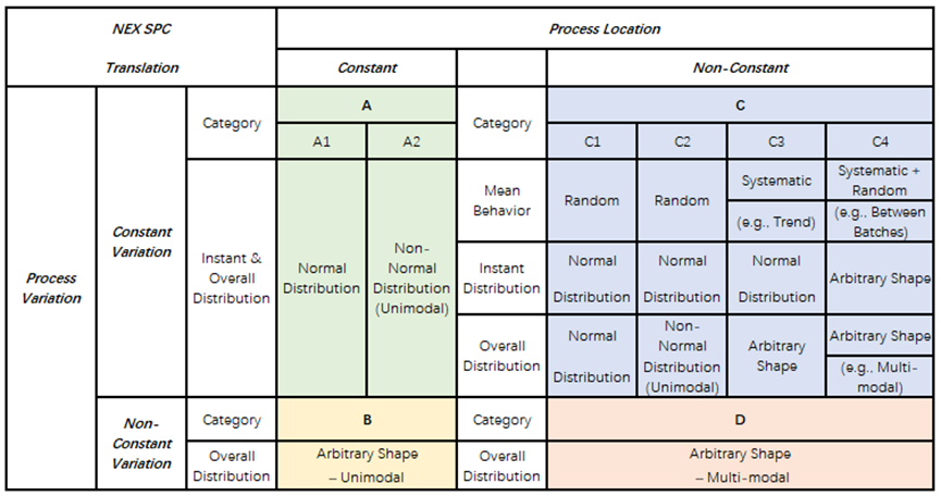
The new standard classifies time-based process distributions into four major categories: A, B, C, and D.
A Simple Way to Understand the Classification
To determine which category a process belongs to, three key aspects must be considered:
- Process variation
- Process location (mean)
- Distribution model
The Four Categories: A, B, C, and D
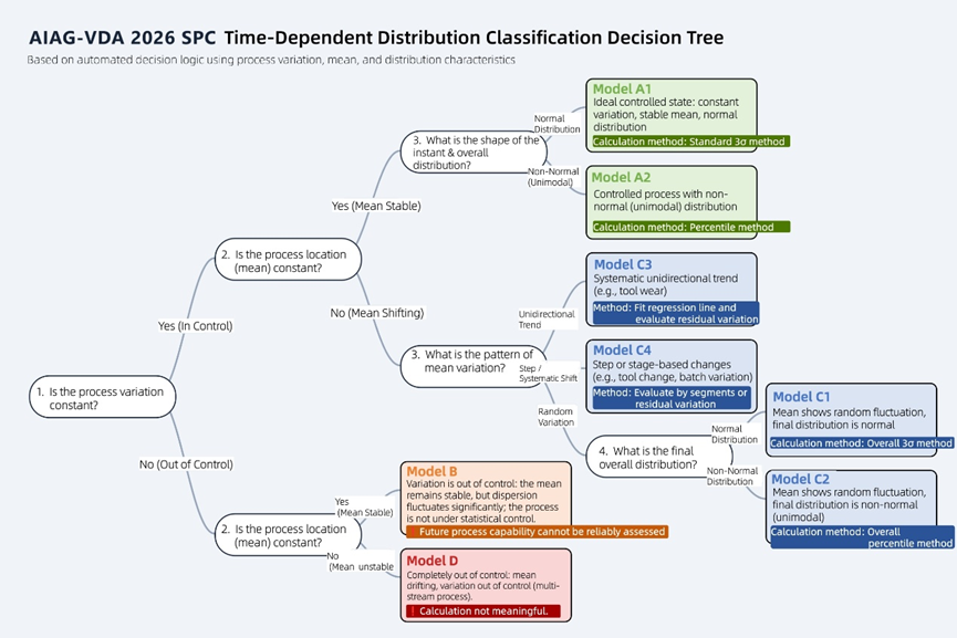
Category A: The “Ideal Student” (Constant Variation, Stable Mean)
Both the variation and the process mean remain stable.
A1 (Normal Distribution)
A textbook-perfect condition. All data points fluctuate around the center line following a normal distribution.
A2 (Non-Normal Distribution)
Although the data does not follow a normal distribution (e.g., surface roughness or roundness constrained by physical limits, often skewed), the process is still stable and under control.
Key point: Stability matters more than normality.
Category C: The “Wanderer” (Constant Variation, Shifting Mean)
This is the most common situation in real production.
The process precision (variation) is stable, but the process mean shifts over time.
C1 / C2 (Random Drift)
The mean fluctuates randomly.
- If the combined result appears normal → C1
- If the combined result is non-normal → C2
C3 (Systematic Trend)
A typical example is tool wear.
As machining progresses, the dimension gradually increases or decreases, forming a clear linear trend.
C4 (Step Change / Shift)
Examples include:
- Tool change
- Material batch change
The process remains stable at one level, then suddenly shifts to another level and stabilizes again, often resulting in a multi-modal distribution.
Category B and D: The “Troublemakers” (Non-Constant Variation)
When variation is not constant (e.g., R chart or S chart out of control), it indicates that the dispersion of the process is unstable.
Category B
The process mean remains stable, but variation fluctuates (e.g., inconsistent spindle wear in multi-spindle machines).
Category D
The worst-case scenario:
- Mean shifts unpredictably
- Variation fluctuates significantly
This represents a chaotic, multi-stream process.
In this condition, calculating Cpk is meaningless and misleading.
Why This Classification Matters
The purpose of dividing time-based models into these categories is to better guide real production decisions.
For example:
If a process is identified as C3 (tool wear trend)
- Traditional Cpk calculations are no longer appropriate
- Capability should be evaluated relative to the trend line
Otherwise, it may lead to incorrect conclusions such as “insufficient capability.”
From Complexity to Automation
The good news is:
You do not need to memorize these complex classification rules or underlying formulas.
NEX SPC will fully support this new AIAG-VDA 2026 classification logic.
The system can:
- Automatically analyze inspection data
- Identify whether the process belongs to A, B, C, or D in seconds
- Automatically apply the most appropriate Cpk/Ppk calculation method based on the classification
Conclusion
The new SPC classification approach shifts the focus from forcing data to fit theoretical assumptions to understanding real process behavior.
By embracing real-world variation, it enables more accurate analysis and more effective quality improvement.
Ultimately, advanced quality standards become practical digital tools that help improve manufacturing yield and process performance.